Data Cleaning in Metabolomics Biomarker Research

Metabolomics Biomarker Series Article Catalog:

1. Unlocking Biomarkers: A Guide to Vital Health Indicators

2. Metabolomics and Biomarkers: Unveiling the Secrets of Biological Signatures

3. Choosing the Right Study Design for Metabolomics Biomarker Discover

4. Metabolomics Biomarker Screening Process

5. Identifying the Right Samples: A Guide to Metabolomics Biomarker Research

6. Data Normalization in Metabolomics Biomarker Research

Welcome back to our ongoing exploration of data preprocessing in metabolomics biomarker research. In our last discussion, we highlighted the importance of data normalization, a critical step in ensuring consistency and comparability across your dataset. By addressing variations in data scale and distribution, normalization sets the stage for more accurate downstream analyses.

As we move forward, our focus shifts to a broader spectrum of data preprocessing tasks encompassed by data cleaning. This next phase includes handling outliers, managing outlier samples, dealing with missing values, and performing batch correction. Each of these steps is essential for maintaining the integrity of your data, minimizing biases, and enhancing the reliability of your results. In the upcoming posts, we will delve into these key aspects of data cleaning, providing you with practical techniques and best practices to refine your metabolomics data. Stay tuned as we continue to unlock the full potential of your research through meticulous data preprocessing.

1. Handling of outliers

Outliers are values in a dataset that have significantly different characteristics from other values, also known as anomalies. Outliers can significantly affect data analysis. Therefore, when encountering a small number of outliers in a dataset, it is generally necessary to accurately screen them out and remove them to avoid interference with the correct results. There are various methods for screening outliers, with box plot and residual analysis being two commonly used methods in metabolomics data processing.

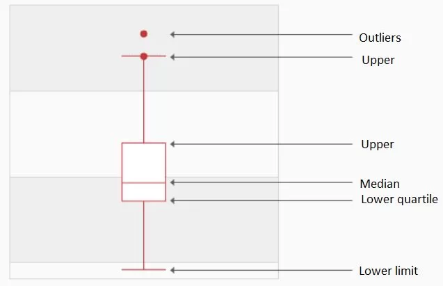A box plot, also known as a box-whisker plot, is a type of statistical chart used to show the dispersion of a set of data. It is named for its box-like shape and is commonly used to quickly identify outliers. The lower quartile in the box plot is Q1, the median is Q2, and the upper quartile is Q3, so the interquartile range IQR = Q3 - Q1. The upper limit is the maximum value within the non-anomalous range - upper limit = Q3+1.5IQR; the lower limit is the minimum value within the non-anomalous range - lower limit = Q11.5IQR. Values that break through the upper and lower limits are considered outliers. The biggest advantage of the box plot is that it is not affected by outliers and depicts the discrete distribution of the data accurately and stably while also facilitating data cleaning.

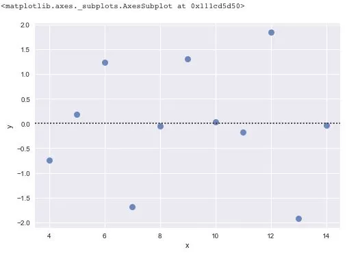There is another method for screening outliers - residual analysis. The so-called residual is the difference between the observed value and the predicted value (fitted value), i.e., the difference between the actual observed value and the regression estimate. In regression analysis, the difference between the measured value and the value predicted by the regression equation is expressed as δ. The residuals δ follow a normal distribution N(0, σ2). (δ - mean of the residual)/standard deviation of the residual is called the standardized residual, which is expressed as δ*. δ* values follow a standard normal distribution N(0, 1). The probability that the standardized residual of an experimental point falls outside the (2, 2) interval is ≤ 0.05. If the standardized residual of an experimental point falls outside the (2, 2) interval, it can be recognized as an outlier experimental point at the 95% confidence level and should be eliminated.

After the outliers are eliminated, they can be treated as missing values, and an appropriate method can be chosen to fill them in.

2. Handling of outlier samples

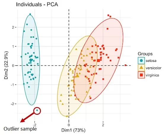When analyzing metabolomics data, we may find some samples with outliers accounting for more than 60%, which indicates that there may be problems with the quality of the sample itself. For example, there may be repeated freezing and thawing, hemolysis, etc., or there may be a large difference between the individual and other individuals in the same group. Such abnormal samples will seriously affect the results of the screening of differential metabolites and should be excluded. Therefore, screening for outlier samples is also highly necessary in data preprocessing. The screening methods we commonly use include PCA and Mahalanobis.

PCA refers to principal component analysis and is a clustering-based outlier detection method. In a PCA score plot, samples within the same group are clustered, with the ellipse representing the 95% confidence interval. Samples falling outside the circle of the group are outlier samples.

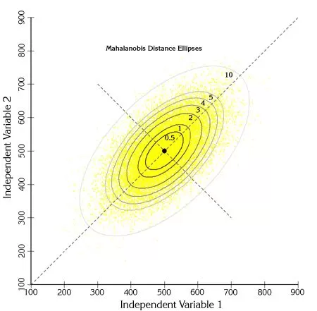Mahalanobis analysis, which refers to the Mahalanobis distance method, is a common method for discriminating multivariate outlier samples based on distance. Mahalanobis distance refers to a distance measure in a multidimensional space, where the size of the distance is evaluated by the distribution, and each sample corresponds to a Mahalanobis distance. First, a critical value needs to be calculated based on the chi-square test, which is related to the test level and the degree of freedom, where the test level is usually set at 0.005 or 0.001. If the Mahalanobis distance for a given sample is greater than the critical value, the individual is considered to be an outlier at test level α.

3. Handling of missing values

3.1 Filtering of missing values

A sample may have one or more missing values for some reason (a. very low signals that are not detected; b. detection errors such as ion suppression or unstable instrument performance; c. limitations of the algorithm used to lift the peaks that did not extract the low signals from the background; d. deconvolution that fails to resolve all of the overlapping peaks). Missing values are usually present in the table as null values or as NA (Not A Number).

Data filtering based on the proportion of missing values within a sample or a group is a commonly used method in metabolomics data analysis. For example, peaks with more than 50% missing in a QC sample are removed, or peaks with more than 80% missing values in a sample are removed.

3.2 Filling of missing values

If the unfiltered missing values are directly ignored, such a data matrix may compromise the computation of subsequent algorithms and will trigger an exception, hence the necessity for simulation filling. A simple method is to fill with a fixed value, mean, median, minimum, or 1/2 minimum; a more complex method is to use machine learning algorithms such as the K-nearest neighbor (KNN), random forest (RF), and singular value decomposition (SVD). The following methods are commonly used in metabolomics data processing:

Filling with a fixed value: A common approach to handle missing feature values is that they can be filled with a fixed value, e.g., 0, 9999, -9999, etc.

Filling with mean, plurality, and median: Filling missing values based on the similarity between samples involves filling them with the most probable values of those missing values. Usually, values that represent the central tendency of the variables are used to fill the missing values. Indicators that represent the central tendency of the variables include the mean, median, plurality, etc. So, which indicators do we use to fill in the missing values?

Mix filling: filling with the minimum value, suitable for missing values due to a metabolite signal response below the instrument detection limit;

Interpolation filling: Interpolation is an important method of discrete function approximation, which can be utilized to estimate the approximation of a function at other points by the values taken by the function at a finite number of points. Unlike fitting, the curve is required to pass through all known data.

Regression filling: Any regression is the process of learning from the feature matrix and then solving for the continuous type label y. This process is made possible because the regression algorithm assumes that there is some association between the feature matrix and the labels before. For data with n features, where the feature T has missing values, the feature T is treated as a label, and the other n-1 features compose a new feature matrix. The part of the T label without missing values and the corresponding part of the new feature matrix are used to predict the missing part of the T label. A common regression model - linear regression - builds regression equations based on the complete dataset. For objects containing null values, the known attribute values are substituted into the equation to estimate the unknown attribute values, and these estimated attribute values are used to fill the missing values.

Random forest filling: The random forest method can also be applied to regression problems, depending on whether each cart tree of the random forest is a classification tree or a regression tree. It makes many put-back samplings from the original dataset, which will result in many different datasets. Then, a decision tree is built for each dataset. The final result of a random forest is averaging the results of all the trees, a new observed value. Through many trees (e.g., n trees), n predicted values are obtained. The average of these n predicted values is eventually used as the final result to fill in the missing values. Of course, just like the preprocessing of the regression data above, the training and prediction sets have to be constructed before the model prediction.

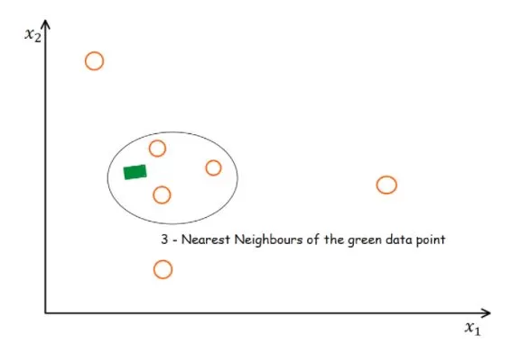KNN filling: It belongs to the algorithm filling. The principle of the KNN method is to identify k samples in the dataset that are spatially similar or comparable. We then use these "k" samples to estimate the values of the missing data points. The missing values for each sample are interpolated using the average of the "k" neighbors found in the dataset.

According to research, the KNN algorithm is the most robust algorithm in the current missing value-filling methods and has been more commonly used in recent years. However, some researchers believe that the choice needs to be made according to the type of missing - completely non-random missing values can be filled using half of the minimum value, and completely random missing or random missing using the random forest method (Wei et al.,2018). Therefore, there is no completely unified standard, and the specific filling method has to be chosen according to the type of data and biological significance.

4. Batch correction

The batch effect, in simple terms, is the experimental error caused by performing the experiment in several batches. The need for correction in metabolomics analysis is due to unstable instruments and other conditions, which may lead to an error in the relative content of the signal peaks.

Batch correction can be further categorized into intra-batch correction and inter-batch correction. There are two typical scenarios for using intra-batch correction: the first is for large projects where metabolite assays can take several days or more than ten days. During this period, the signal strength of metabolites will fluctuate at different levels, resulting in errors in the quantitative data of metabolites, thus requiring correction. The second scenario is that for small and medium-sized projects under special conditions. Intra-batch correction is not necessary for routine small and medium-sized projects. However, intra-batch correction is particularly important if there is a sudden instrument malfunction, power failure, or other special circumstances during the operation of a project. Inter-batch correction is usually carried out due to the difficulties in collecting clinical samples over a long period of time. In order to avoid changes in metabolites caused by the prolonged storage of samples, metabolomics assays are carried out in batches. Finally, all the data are integrated and analyzed by using batch correction. While batch correction may improve the batch effect to some extent, it does not eliminate the batch effect completely. It is, therefore, not recommended to test in batches if an alternative solution is available.

The QC-mix sample-based correction is usually chosen among the batch correction methods for metabolomics data. A QC-mix consists of a mixture of all samples or a randomly selected proportion of samples taken in equal parts. During mass spectrometry, a QC-mix sample is injected every a certain number of samples. Since the QC-mix samples are identical, they can be used to simulate the changes in the signal during data acquisition. After obtaining the data, the QC-mix samples are used as a training set for each metabolite to build a prediction model to predict the signal change and thereby correct the sample signals.

The commonly used batch correction methods in metabolomics can be categorized into two types based on the source, which are:

metaX (Wen et al. 2017):

SVR (Support Vector Regression) (Shen et al., 2016)

RSC (Robust Spline Correction) (Kirwan et al., 2013)

combat (Johnson, Li, and Rabinovic 2007)

statTarget (Luan et al. 2018a; Luan et al. 2018b):

QC-RFSC (QC-based random forest signal correction)

QC-RLSC (QC-based robust LOESS signal correction)

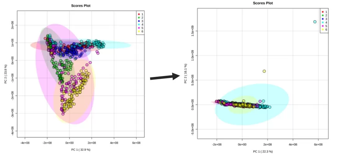
When carrying out batch correction for an actual project, we can try a variety of correction methods and combine them with specific data to conduct multiple tunings in order to achieve the desired effects.

Reference:

[1] Johnson, W. Evan, Cheng Li, and Ariel Rabinovic. 2007. “Adjusting Batch Effects in Microarray Expression Data Using Empirical Bayes Methods.” Biostatistics 8 (1): 118–27. doi:10.1093/biostatistics/kxj037.

[2] Kirwan, J. A., D. I. Broadhurst, R. L. Davidson, and M. R. Viant. 2013. “Characterising and Correcting Batch Variation in an Automated Direct Infusion Mass Spectrometry (DIMS) Metabolomics Workflow.” Analytical and Bioanalytical Chemistry 405 (15): 5147–57. doi:10.1007/s00216-013-6856-7.

[3] Luan, Hemi, Fenfen Ji, Yu Chen, and Zongwei Cai. 2018a. “Quality Control-Based Signal Drift Correction and Interpretations of Metabolomics/Proteomics Data Using Random Forest Regression.” bioRxiv, January, 253583. doi:10.1101/253583.

[4] ———. 2018b. “statTarget: A Streamlined Tool for Signal Drift Correction and Interpretations of Quantitative Mass Spectrometry-Based Omics Data.” Analytica Chimica Acta 1036 (December): 66–72. doi:10.1016/j.aca.2018.08.002.

[5] Shen, Xiaotao, Xiaoyun Gong, Yuping Cai, Yuan Guo, Jia Tu, Hao Li, Tao Zhang, Jialin Wang, Fuzhong Xue, and Zheng-Jiang Zhu. 2016. “Normalization and Integration of Large-Scale Metabolomics Data Using Support Vector Regression.” Metabolomics 12 (5): 89. doi:10.1007/s11306-016-1026-5.

[6] Wen, Bo, Zhanlong Mei, Chunwei Zeng, and Siqi Liu. 2017. “metaX: A Flexible and Comprehensive Software for Processing Metabolomics Data.” BMC Bioinformatics 18 (1): 183. doi:10.1186/s12859-017-1579-y.