Data Preprocessing in Metabolomics Biomarker Research

Metabolomics Biomarker Series Article Catalog:

1. Unlocking Biomarkers: A Guide to Vital Health Indicators

2. Metabolomics and Biomarkers: Unveiling the Secrets of Biological Signatures

3. Choosing the Right Study Design for Metabolomics Biomarker Discover

4. Metabolomics Biomarker Screening Process

5. Identifying the Right Samples: A Guide to Metabolomics Biomarker Research

Welcome back to our series on metabolomics biomarker research! In our previous posts, we delved into the intricacies of designing robust experiments in the quest to uncover valuable biomarkers. We discussed how careful planning, including study type selection, screening process definition, sample selection, control groups, and variable management, forms the bedrock of credible and reproducible metabolomics research. Now, as we transition to the next phase of our journey, we turn our attention to a crucial step that follows meticulous experiment design: data preprocessing.

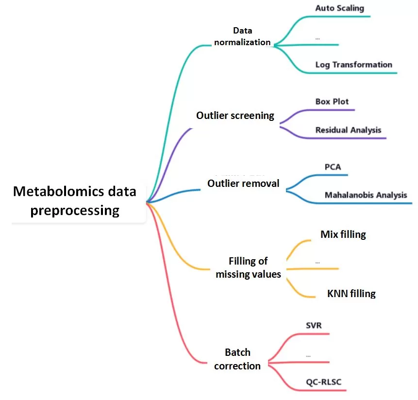
Data preprocessing is the bridge between raw experimental data and meaningful biological insights. The raw metabolomics data contains quality control (QC) samples and test samples. In order to better analyze the data, a series of preprocessing of the raw data is required, which mainly includes normalization of the raw data, screening of outliers, processing of outlier samples, and filling of missing values. Data pre-processing can reduce the impact of variants in the data that are not relevant to the purpose of the study on data analysis, facilitating the screening and analysis of potential target differential metabolites.

In the upcoming posts, we will delve into the various techniques and best practices for preprocessing metabolomics data, setting the stage for accurate and insightful biomarker discovery. To begin, we will introduce the critical process of data normalization.

Data normalization is also called data standardization by some scholars. The main purposes of data normalization include: 1) to make the data dimensionless so that variables of different natures are comparable; 2) to transform the data of different orders of magnitude to a suitable range, avoiding the fluctuation of small-value variables masked by large-value variables; 3) to make the overall data conform to the normal distribution, so as to facilitate parameter testing; 4) in addition, data normalization allows a uniform distribution of data, facilitating the plotting and presentation of data, and so on.

1. Definition of data normalization

Data normalization in metabolomics refers to a series of centering, scaling, and transforming operations on quantitative data from multiple samples and metabolites, with the aim of reducing noise interference in the dataset, emphasizing the biological information, making it amenable to subsequent statistical analyses, and improving the interpretability of its biological properties.

Simply put, some changes are made to the metabolic dataset to pull the data into a specific range and make it more statistically significant.

2. The necessity of data normalization

Let's illustrate this by coming to an actual dataset:

Note: These data come from a subset of our actual project data, which has been subjected to data masking. Metabolite ID.

It can be clearly seen that the above metabolic data share the typical characteristics of high dimensionality, high noise, etc., and that there are generally order-of-magnitude differences between different metabolites or samples. For example, the metabolite MW0006, which is highlighted in the table, differs more than 1,000-fold in 6 samples and does not have a disproportionate biological relevance to Met0008. In addition, many statistical analysis methods are sensitive to the distribution of the data, with the statistical power usually focused on those metabolites with high concentrations or large fold changes. However, it is likely that those metabolites with low concentrations are the ones that really make a difference. Therefore, it is necessary to carry out reasonable data normalization for different statistical analysis methods.

3. Data normalization methods

The common methods used in omics analysis can be broadly grouped into the following three categories:

• Centering: i.e., subtracting the mean value from all data so that the data are distributed around the 0 value instead of around the mean value, focusing on the differences in the data;
• Scaling: refers to uniformly multiplying or dividing data by a factor to eliminate order-of-magnitude differences, and there are a variety of scaling methods adapted to different analytical needs;
• Transformation: i.e., performing Log or Power transformations to eliminate heterogeneity.

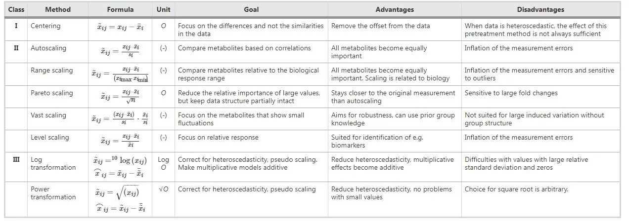
These three methods were summarized by Berg et al. in 2006:

They are explained and supplemented below:

• Centering: It refers to transforming data from near the mean to near the 0 value. It is not effective in handling data with heteroskedasticity; 
• Auto Scaling: It's often termed as zero-value normalization, Z-score normalization, or UV (unit variance scaling), etc.; It turns the data into a dataset with a mean of 0 and a variance of 1, concentrating the variations on the correlation between metabolites; It is sensitive to noise signals and is widely used in many machine learning algorithms (e.g., support vector machine, logistic regression, and artificial neural network analysis); 
• Min-Max Scaling: deviation normalization, scales data to the [0,1] interval, and is sensitive to outliers; 
• Range Scaling: It computes the ratio of change volume to change range and the direction of change; It is sensitive to measurement errors and outliers; 
• Pareto Scaling: It preserves the original structure of the data to a certain extent compared to Auto Scaling, giving results that are closer to the original data, but is more sensitive to large multiplicative differences; 
• Vast Scaling: It focuses on metabolites with small variations and requires specific populations for better results. It allows for supervised analysis; 
• Level Scaling: It compares the change volume relative to the mean; It’s suitable for biomarker discovery and is sensitive to errors; 
• Log Transformation: It eliminates the effects of heteroscedasticity and large multiplicative differences, and linearizes the data; Metabolomics data generally show a skewed distribution (right skewed) and, therefore, require a suitable transformation to make the data distribution more symmetrical. If there are 0 or negative values in the data, a number can be added to all data to convert such values to positive numbers, so log(1+x) is commonly used; 
• Power Transformation: It eliminates the effect of heteroscedasticity and linearizes the data. It is important to choose the right root. 
• Total Peak Area Normalization: The value of a single metabolite in a single sample/sum of all metabolites in that sample, i.e., the calculation is done by converting the absolute value of the content into the proportion of each metabolite to the total metabolite content in the sample. This method is commonly used for urine metabolomics normalization.
• Common Peak Area Normalization: The value of a single metabolite in a single sample / the sum of the metabolites in all samples. This method increases the accuracy of the normalization compared to total peak area normalization by eliminating the interference of specific variables with available signal peaks that are only present in individual samples.
• Creatinine Normalization: Creatinine is a low molecular weight nitrogenous substance. The amount of creatinine excreted in the urine per day by a normal organism is constant and is not affected by factors such as urine volume. It is, therefore, often used as a calibrator in urinary metabolomics studies, i.e., the peak area of each variable is divided by the corresponding peak area of creatinine.
• PQN: Probabilistic Quotient Normalization, is also a commonly used method for normalizing urine metabolomics data. The premise assumption of this algorithm is that most metabolites are constant from sample to sample, and only some are differentially expressed. It is not applicable to datasets with a large number of differentially expressed metabolites.

4. Selection of normalization methods

As we mentioned earlier, some statistical analyses are very sensitive to normalization methods, with PCA analysis being a prime example. In the next section, we will perform different normalizations on two actual datasets followed by PCA analysis so that we can have a look at the effect of different methods. (The data are from one of our actual projects. Information such as metabolite ID, sample name, group name, etc., have been masked, and part of the data has been deleted.)

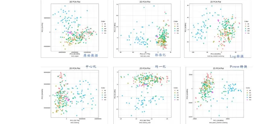
The figure below shows the results obtained from the five most commonly used methods in metabolomics data analysis.

Dataset 1 is divided into 2 groups and 3 geographic groups, totaling 221 samples plus 13 mixes, with 600+ metabolites detected.

There are four sample groups and one mix group in the figure above. In the sample groups, AE (orange), AS (olive), and AW (green) are samples of the same group in different geographic areas; BW (blue) is another group but in the same geographic area as AW; and the mix group (pink) should be clustered into a single point. Auto-scaling (normalization) and both transformation methods are clearly working better, as can be seen in the above figure.

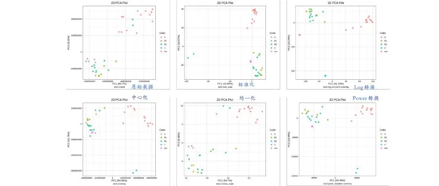
Dataset 2 consists of a total of 31 samples from multiple individuals and different tissues plus 3 mixes, with 600+ metabolites detected.

There are a total of four sample groups and a mix group in the above figure. A (orange) is a tissue; B1 (olive) and B2 (green) are different sites of the same tissue; C (blue) is another tissue; the mix group (pink) should be clustered into a single point. It can be seen from this figure that, again, the auto-scaling (normalization) and the two transformation methods are obviously more effective, of which the Log transformation approach is the most effective. In an article published in 2018, Li Shuang [2] counted the most used normalization method in the metabolome-related literature, which is Log transformation. It is evident that the Log transformation method is the one with the most adaptability.

The two transformation methods and the auto-scaling method gave excellent results for two different sets of data. Although it does not represent the full extent of metabolomics data, it is a good indication of the effectiveness of these three methods. In addition, in the figures that are not shown here, Pareto scaling gives comparable results to the auto-scaling method, followed by the range scaling method.

In fact, it is not advisable to choose the method to be used from the results because the reason for better results, regardless of the method, is based on the intrinsic characteristics of the metabolomics data. Typical widely-targeted metabolomics and untargeted metabolomics data are characterized by high dimensionality, high noise, sparse, and right-skewed. PCA requires the data to be homoskedastic, is sensitive to heteroskedasticity, and is sensitive to linearity. The above-mentioned normalization methods with better performance are only suitable for PCA. If a different statistical method is used, the normalization method should be adjusted accordingly. Therefore, when analyzing the data, we can try several normalization methods, followed by repeated tuning in conjunction with the specific experimental content and objectives, in order to achieve the desired goals.

References:

[1] van den Berg, R.A., Hoefsloot, H.C., Westerhuis, J.A. et al. Centering, scaling, and transformations: improving the biological information content of metabolomics data. BMC Genomics 7, 142 (2006).

[2] Li Shuang, Comprehensive evaluation of metabolomics-based data normalization methods [D]. Chongqing University,2018.