Non-negative Matrix Factorization (NMF) for Omics: A Practical, Interpretable Guide

Non-negative Matrix Factorization (NMF) is a parts-based matrix decomposition that turns non-negative omics data into interpretable modules. In bioinformatics, NMF (and cNMF) enables feature extraction in transcriptomics—bulk and single-cell RNA-seq—as well as proteomics and metabolomics, revealing latent gene programs and per-sample usage scores for biomarker discovery, patient stratification, and modular analysis. This practical guide explains V≈WH, rank k selection, consensus stabilization, and enrichment/validation, with real-world case studies and code to get started. If you need an interpretable alternative to PCA/ICA, NMF provides additive, sparse patterns that map cleanly to biology.

Why Decompose Complex Biological Data?

In biology, most signals don’t subtract—they add up. That’s why Non-negative Matrix Factorization (NMF) often feels more “biological” than PCA: it explains a sample as a recipe of non-negative building blocks—gene programs that we can name, score, and test. If omics matrices are mixtures (like a symphony’s instruments or a milk tea’s ingredients), NMF helps “take apart the mix” into interpretable parts that map to pathways, cell states, and microenvironment signals.

NMF in One Minute (V≈WH): What W and H Mean—and Why Non-negativity Matters

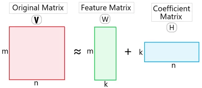
Given a non-negative matrix V ∈ ℝ₊^{m×n} (e.g., genes × samples/cells), NMF finds non-negative matrices
W ∈ ℝ₊^{m×k} (basis; columns ≈ gene programs) and
H ∈ ℝ₊^{k×n} (coefficients; rows ≈ program usage per sample/cell)
such that V ≈ W H. Because all entries are non-negative, patterns add rather than cancel, yielding parts-based, often sparse modules that map cleanly to biology—unlike PCA loadings with positive/negative signs.

How to read W and H: Use W to name programs (top genes + enrichment), and H to score each sample/cell.

For example, a face image (V) can be decomposed into local parts (W: eyes, nose, mouth) and their mixing weights (H). The full face is reconstructed by additively combining these parts.

NMF vs PCA vs ICA: A Pocket Decision Guide

Tip: If downstream stakeholders want named pathways and per-sample scores, start with NMF; keep PCA as a QC/visualization companion.

An Omics-Ready Workflow (QC → Rank k → Fit → cNMF → Enrichment → Validate)

1. Pre-process & QC

Filter low-abundance features; normalize counts (e.g., CPM/TPM or variance-stabilizing transforms for RNA-seq); correct batch effects. For scRNA-seq, remove low-quality cells/doublets and address sparsity.

2. Choose rank k (try a grid like 5–50)

Track reconstruction error (elbow), stability (consensus/cophenetic), sparseness, and biological enrichment (GO/KEGG/Reactome). Prefer the smallest k that is stable, sparse, and coherent.

3. Fit NMF

Loss: Euclidean (least squares) or KL divergence for count-like data

Initialization: NNDSVD or multiple random starts

Optimizers: multiplicative updates, projected gradients, or coordinate descent

4. Stabilize with consensus NMF (cNMF)

Run NMF many times, cluster factors, and derive consensus programs to mitigate local minima and noise.

5. Interpret factors

Rank top genes per program (columns of W); annotate via pathway enrichment and known signatures. Link program scores (rows of H) to phenotypes (subtypes, stage, response) and metadata.

6. Validate & deploy

Reproduce programs via resampling or external cohorts. Build program-score classifiers or risk models and test on hold-out datasets.

Selecting k: Error, Stability, Sparseness, Biology

Error elbow: look for diminishing returns in reconstruction error.

Stability: consensus/cophenetic remains high across seeds/subsamples.

Sparseness: crisper gene sets aid interpretation and panel design.

Biology: programs enriched for coherent pathways; align with known subtypes.

Generalization: program scores predictive in external data.

Rule of thumb: Don’t chase larger k. The most explainable, reproducible k wins.

Applications of NMF

Biomedicine: decoding gene programs

Gene-expression data typically form matrices (genes × samples). NMF helps uncover structure such as:

Tumor subtype identification: Factorization exposes latent patterns that delineate molecular subtypes, aiding biomarker discovery.

Single-cell analysis: In scRNA-seq, NMF extracts cell-type features and gene modules for downstream classification and modular analysis.

NMF thus acts like a conductor, separating noisy expression into clearer “melodies.”

Image and signal processing

Face recognition: Early methods used NMF to represent faces as local parts (eyes, nose, mouth).

Music separation: Mixed audio can be decomposed into vocals and accompaniment.

Image compression/denoising: Main features are retained while redundancy is reduced.

Recommender systems

For user-item rating matrices, NMF yields:

W: user preference features;

H: latent attributes of items.

This supports rating prediction and personalized recommendations.

Text mining

In document–term matrices, NMF performs topic modeling:

W (topic × term): terms defining each topic;

H (document × topic): topic proportions per document.

Real-World Examples: NMF in single-cell data

In scRNA-seq, cells typically express mixtures of identity (cell type) and activity (state) programs. Building on the notation above, cNMF stabilizes program discovery across seeds/subsamples. We illustrate two representative applications below.

Parsing intratumoral transcriptional heterogeneity with NMF

Intratumoral heterogeneity (ITH) arises from genetic, epigenetic, and microenvironmental drivers and influences treatment failure, metastasis, and other phenotypes. scRNA-seq profiles ITH across many cancers.

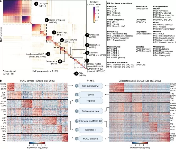
In “Hallmarks of transcriptional intratumour heterogeneity across a thousand tumours,” the authors annotated cell types and copy-number variation across 1,456 samples from 77 studies (24 cancer types; 2,591,545 cells), identifying over 680,000 malignant cells and roughly 120 non-malignant cells. NMF applied to malignant cells characterized ITH; similar modules were merged into 41 malignant programs (MPs) with associated gene sets.

Pan-cancer scRNA-seq workflow: NMF-derived heterogeneity programs and consensus meta-programs (MPs) [3]

Functional enrichment grouped these into 11 MP families. The most prevalent involved the cell cycle (MP1–4), stress/hypoxia (MP5–7), and mesenchymal (MES)/EMT-like states (MP12–16). Multiple MPs within a family reflected variation within related processes—for example, beyond canonical G2/M and G1/S MPs (MP1 and MP2), two less common MPs emphasized HMG-box proteins (MP3) or chromatin regulators (MP4). Mesenchymal/EMT-like MPs varied in cancer-type specificity; a “mixed” program (MP14) included both mesenchymal and epithelial markers. Intermediate-frequency MPs resembled known ITH patterns (protein regulation, interferon response, EpiSen, cilia). Low-frequency MPs (<1% of all NMF programs) were lineage-specific (e.g., neural or hematopoietic) and were merged by lineage.

Pan-cancer NMF meta-programs: similarity map and sample heatmaps [3]

Using NMF to decompose cellular programs

NMF and consensus NMF (cNMF) are widely used to extract cell-identity and activity programs as gene modules. NMF unbiasedly decomposes profiles into a gene-feature matrix (W) and a cell-feature matrix (H).

In “Single-cell transcriptome landscape of circulating CD4+ T cell populations in autoimmune diseases,” NMF decomposed peripheral CD4+ T-cell programs into 12 components aligned with T-cell polarization and differentiation. Examples include Treg-Feature (Treg-F) and Th17-F, each linked to specific transcription factors and functions.

NMF programs in circulating CD4+ T cells: 12 gene-program signatures (heatmap overview) [4]

Based on the top 10 genes per feature and prior studies, the 12 features were named: NMF0 cytotoxic feature (F), NMF1 Treg-F, NMF2 Th17-F, NMF3 naïve feature, NMF4 activation feature (Act), NMF5 TregEff/Th2-F, NMF6 Tfh-F, NMF7 interferon feature (IFN), NMF8 central-memory feature, NMF9 thymic-emigrant feature, NMF10 tissue feature, and NMF11 Th1 feature.

Strengths, Limitations, and Mitigations of NMF in Bioinformatics

Strengths

• Interpretability: Additive, parts-based modules that align with pathways and cell states; easy to name and score across samples/cells.
• Fit for omics sparsity: Works well on high-dimensional, non-negative, sparse matrices (bulk & single-cell).
• Modular analytics: Concise gene programs support biomarker discovery, risk modeling, and cross-cohort transfer.

Limitations & Mitigations

Rank sensitivity (choose k) → Grid-search k with reconstruction error elbow, consensus stability, sparseness, and biological enrichment; prefer the smallest coherent k. (See “Selecting k”.)

Non-uniqueness / local minima → Run cNMF (many inits/subsamples), cluster factors, and take consensus; use NNDSVD init and compare Euclidean vs. KL loss. (See “Workflow” & “cNMF”.)

Noise & batch effects → Rigorous QC (filter low-quality cells/genes), batch correction/integration, and external validation of program scores. (See “Pre-process & QC” and “Validate”.)

Rule of thumb: aim for the most explainable and reproducible

k, stabilize with cNMF, and validate programs out-of-sample.

Extensions that Matter in Practice

Sparse/regularized NMF: L1/L2 penalties encourage concise, high-contrast programs (useful for biomarker discovery).

Semi-supervised / constrained NMF: incorporate prior pathways/signatures to steer factors.

Graph-regularized NMF (GNMF): incorporate gene–gene or cell–cell graphs to respect manifold structure during factorization.

Joint/multi-omics NMF: share programs across transcriptomics/proteomics/metabolomics while allowing modality-specific components.

Deep/hybrid NMF: layer NMF with neural nets for hierarchical parts.

cNMF pipeline: robust default for scRNA-seq program discovery.

FAQ: Practical Answers for Running NMF in Omics

Q1: What is NMF in bioinformatics?
A non-negative matrix factorization of omics data that yields gene programs (W) and usage profiles (H) for modular analysis, feature extraction, and biomarker discovery.

Q2: How do I choose k?
Scan multiple k values; pick the smallest that balances error, consensus stability, sparseness, and pathway coherence—then validate on external data.

Q3: NMF vs PCA for transcriptomics?
Prefer NMF when you need additive, interpretable parts for non-negative counts; keep PCA for variance exploration/QC in Euclidean space.

Q4: Can I use NMF for single-cell RNA-seq?
Yes. cNMF robustly extracts cell-identity and activity programs and their per-cell usage, complementing clustering and trajectories.

Q5: Which loss function should I pick?
KL divergence often suits count-like data; Euclidean works well for transformed/normalized matrices—compare both in practice.

Try It (10-Line Starter in Python)

import numpy as npfrom sklearn.decomposition import NMFfrom sklearn.preprocessing import normalize

# V: genes x samples (non-negative). rows=genes, cols=samples/cells

V = np.load("expression.npy")  # placeholder

V = np.nan_to_num(V)           # simple hygiene

k = 20  # candidate rank

model = NMF(

n_components=k,

init="nndsvd",

solver="cd",

beta_loss="kullback-leibler",

max_iter=500,

random_state=1

)

W = model.fit_transform(V)  # genes x k (programs)

H = model.components_       # k x samples (usage)

W = normalize(W, axis=0)    # optional: column-normalize for easy top-genes

Next: repeat with different seeds, cluster factors for cNMF, then enrich top genes per program (GO/KEGG/Reactome).

Conclusion

NMF is a practical key for decoding complex, non-negative data:

• It expresses massive datasets as understandable basis components.
• It supports applications from biomedicine and text mining to recommender systems and signal processing.
• Its strengths are interpretability and modular analysis; challenges include rank selection and solution stability.

As methods and computing improve, NMF will continue to clarify complex omics data—advancing feature extraction in transcriptomics and downstream analyses in bioinformatics.

References

1. Lee DD, Seung HS. Learning the parts of objects by non-negative matrix factorization. Nature. 1999;401:788–791.
2. Kotliar D, et al. Identifying gene expression programs of cell-type identity and cellular activity with cNMF. eLife. 2019;8:e43803.
3. Gavish A, Tyler M, Greenwald AC, et al. Hallmarks of transcriptional intratumour heterogeneity across a thousand tumours. Nature. 2023;618:598–606. doi:10.1038/s41586-023-06130-4.
4. Yasumizu Y, Ohkura N, Sakaguchi S, et al. Single-cell transcriptome landscape of circulating CD4⁺ T-cell populations in autoimmune diseases. Cell Genomics. 2024;4(1):100454.
5. Cai D, He X, Han J, Huang TS. Graph Regularized Non-negative Matrix Factorization for Data Representation. IEEE TPAMI. 2011.

Read more

• Metabolomic Analyses: Comparison of PCA, PLS-DA and OPLS-DA
• WGCNA Explained: Everything You Need to Know
• Harnessing the Power of WGCNA Analysis in Multi-Omics Data
• Beginner for KEGG Pathway Analysis: The Complete Guide
• GSEA Enrichment Analysis: A Quick Guide to Understanding and Applying Gene Set Enrichment Analysis
• Comparative Analysis of Venn Diagrams and UpSetR in Omics Data Visualization
• Metabolomics Batch Effects