LC–MS/MS Proteomics Data Analysis: From Raw Files to Publication-Ready Results

Proteomics is a core approach for studying biology at the functional protein level, enabling applications from biomarker discovery to mechanism-driven research. Modern high-resolution LC–MS/MS proteomics routinely generates large, high-dimensional datasets, making proteomics data analysis the decisive step for translating instrument signals into reproducible peptide/protein identifications, quantitative comparisons, and biologically defensible conclusions. This blog provides a concise, practical roadmap of the LC–MS/MS proteomics analysis pipeline, helping readers move from raw spectra to publication-ready results and mechanism-level insights with greater consistency and confidence.

1. LC–MS/MS Data Processing Basics: From Raw Files to Peptide Features

Reliable proteomics results begin with transforming raw LC–MS/MS files into clean, analysis-ready signals. That foundation—file conversion, peak detection, and feature extraction—largely determines data quality and sets the ceiling for downstream identification depth and quantitative accuracy.

1.1 Raw File Conversion to mzML: Standardization for Proteomics Analysis

Raw files generated by mass spectrometers (for example, Thermo Scientific Orbitrap instruments) are typically stored in vendor-specific binary formats such as .raw. These formats capture rich information, including spectral traces, scan metadata, and instrument settings, but their proprietary nature can limit cross-platform compatibility and reduce transparency for reproducible analysis. For this reason, a standard first step in LC–MS proteomics data processing is converting vendor files into open formats, most commonly mzML or mzXML, which are broadly supported across open-source and commercial software ecosystems.

ProteoWizard is widely used for raw-file conversion, and msConvert is considered an industry-standard utility for exporting vendor formats into mzML. It supports raw data from major instrument vendors and provides filters that make downstream identification and quantification workflows more robust. Core functions and parameters include:

1) Format conversion: The simplest conversion command is msconvert original_file.raw --mzML, which generates a standard mzML output for downstream processing.

2) Data compression: zlib compression can substantially reduce file size, improving long-term storage and transfer efficiency without changing the underlying information content.

3) Centroiding / peak picking: Centroiding converts profile-mode spectra into peak lists by summarizing isotopic peak shapes into representative centroid m/z values and integrated intensities. This step reduces data volume and is often required for efficient database search and DIA processing. In msConvert, centroiding can be enabled using filters such as --filter "peakPicking true [1,2]", where [1,2] indicates applying peak picking to MS1 and MS2 scans.

4) Vendor algorithms: When available, vendor peak-picking algorithms (for example Thermo’s native centroiding) often perform better than generic implementations, particularly for complex spectra. In msConvert, this can be enabled with --filter "peakPicking vendor".

5) Zero-value sample removal: Removing redundant zero-intensity points using --filter "zeroSamples removeExtra" can further optimize file size and improve computational efficiency in later steps.

ProteoWizard uses modern design principles to implement a modular framework of many independent libraries grouped in dependency levels with strict interfaces (Chambers et al., 2012, Nature biotechnology).

As a practical baseline for most workflows, it is recommended to use an up-to-date msConvert release, apply vendor centroiding, and export .raw files into centroided mzML. This improves interoperability with common downstream tools (for example DIA-NN and OpenMS) and provides a clean starting point for feature detection, identification, and quantification.

1.2 Feature Extraction in Proteomics: Peak Detection and Deconvolution

Feature extraction aims to identify signals in converted MS data that truly represent peptide ions (or intact proteins) and to assign their key attributes such as accurate m/z, charge state, intensity, retention time behavior, and isotopic patterns. The exact focus varies by experiment type: bottom-up proteomics emphasizes peptide-level peaks and chromatographic features, while top-down proteomics and intact protein workflows often require explicit deconvolution of charge envelopes. (Learn more at: Top-Down vs. Bottom-Up Proteomics)

Centroiding and Peak Picking for Peptide-Level Signals

In conventional bottom-up proteomics, peak detection is often completed during conversion through centroiding. The core goal is to correctly recognize isotopic peaks, calculate centroid m/z values, and obtain intensity metrics suitable for peptide identification and quantification.

Signal extraction quality is strongly influenced by two parameters. First, the signal-to-noise ratio (S/N) is essential for separating true ion signals from baseline noise; peaks below typical thresholds (for example S/N 3–5) are often unreliable. Second, instrument resolution (for example 120,000 at m/z 200 on an Orbitrap) determines peak width and separation. Peak-picking algorithms must respect these settings to avoid merging adjacent peaks or splitting true peaks incorrectly.

Intact Protein Deconvolution: Charge States to Neutral Mass

In top-down or intact protein MS, a single protein often appears as a distribution of multiple charge states, forming an isotopic envelope that is not directly interpretable as molecular mass. Deconvolution resolves this charge-state pattern and converts it into a neutral (zero-charge) mass representation, enabling intact mass profiling and downstream interpretation.

A commonly used option is Thermo Protein Deconvolution, which provides algorithms such as ReSpect™ and Xtract. ReSpect™ is fast and robust for relatively clean, high-abundance spectra, whereas Xtract offers finer control and can resolve more complex situations, including overlapping species and weaker signals. For open-source analysis environments, Orbitool can also support Orbitrap data processing and certain deconvolution-related tasks.

In practice, deconvolution quality depends on setting appropriate ranges and models. Users typically specify the algorithm (ReSpect™ or Xtract), define a reasonable charge-state range, set an expected mass range (for example 10,000–100,000 Da), and select an appropriate peak model reflecting intact protein behavior and instrument resolution. Noise-related thresholds (including S/N and noise compensation) help reduce false positives, while sliding windows or tolerance parameters guide the search across m/z space. Algorithm selection is ultimately data-driven. When spectra are simple and signals are strong, ReSpect™ is often sufficient. For mixtures, low-abundance proteins, or heavily modified species, Xtract may provide more reliable resolution, although parameter tuning is often required to achieve optimal results.

2. Protein Identification and Quantification: DDA and DIA Workflows

After preprocessing and feature extraction, proteomics analysis focuses on two central tasks: identification (assigning peptide/protein identities to signals) and quantification (measuring abundance across samples). At this stage, the acquisition strategy—DDA vs DIA—largely determines the computational workflow, software tools, and typical sources of missingness or interference.

2.1 Data-Dependent Acquisition (DDA) Proteomics Workflow

Data-dependent acquisition (DDA), often referred to as shotgun proteomics, selects precursors for fragmentation based on MS1 intensity. The instrument performs an MS1 survey scan, ranks precursor ions, isolates the top N precursors (for example Top10–Top20), fragments them (CID or HCD), and records MS2 spectra for identification.

DDA Database Search Engines: Key Settings and FDR Control

DDA identification relies on matching experimental MS2 spectra to theoretical spectra derived from a protein sequence database. Common search platforms include MaxQuant/Andromeda, Proteome Discoverer/SEQUEST HT, and Mascot, each implementing its own scoring, filtering, and reporting conventions.

Search quality depends on properly setting key parameters. The protein database is typically FASTA-formatted (for example UniProt/Swiss-Prot or NCBI RefSeq) and must match the sample species to avoid inflated false matches. Enzyme settings commonly use Trypsin/P, allowing a limited number of missed cleavages (often 1–2). High-resolution instruments typically support tight precursor mass tolerances (for example 10–20 ppm), while fragment mass tolerance depends on the MS2 analyzer (high-resolution Orbitrap values such as 20 ppm or 0.02 Da, versus wider tolerances for ion trap detection).

Chemical modifications are generally separated into fixed modifications (for example carbamidomethylation of cysteine) and variable modifications (for example methionine oxidation or protein N-terminal acetylation). Finally, confidence is controlled using false discovery rate (FDR), most often estimated through a target–decoy strategy, with typical thresholds of 1% at both the PSM and protein levels.

DDA Quantification Strategies: LFQ vs TMT/iTRAQ Proteomics

DDA quantification is commonly performed using either label-free quantification (LFQ) or isobaric labeling such as TMT/iTRAQ proteomics.

In LFQ workflows, relative abundance is inferred by comparing MS1 intensities (peak areas or heights) for the same peptide across runs. MaxQuant MaxLFQ is widely used because it integrates multiple peptide ratios through a global optimization framework to produce stable protein-level quantification. Parameters that often matter in practice include enabling LFQ, choosing an appropriate minimum ratio count, and using Match Between Runs, which transfers identifications across runs based on accurate mass and retention time alignment. When chromatography is stable, this feature can reduce missing values and substantially improve coverage.

In contrast, TMT/iTRAQ workflows label peptides from different samples with isobaric tags, mix them, and quantify reporter ions released during fragmentation. While MS1 signals are merged, reporter ion intensities in MS2 (or MS3) encode relative abundance. Because reporter ions are sensitive to co-isolation interference, advanced TMT experiments often use SPS-MS3 to improve quantitative accuracy by generating cleaner reporter ion spectra. In MaxQuant, this is typically configured by selecting reporter ion MS2 or MS3 modes and specifying the correct TMT plex type.

2.2 Data-Independent Acquisition (DIA) Proteomics Workflow

Data-independent acquisition (DIA), including SWATH-style methods, fragments all ions within sequential wide m/z windows across the LC gradient. This produces highly information-rich data and supports consistent quantification because peptides are measured more systematically than in DDA. However, DIA MS2 spectra are multiplexed mixtures of fragments from many precursors, so traditional DDA-style spectrum-by-spectrum searching is not directly applicable.

Spectral Library DIA: XIC Extraction, Scoring, and FDR Control

A mainstream DIA strategy is spectral library-based DIA, where peptide detection and quantification are guided by a library containing expected precursor m/z, fragment patterns, and retention time anchors (often iRT).

Libraries can be built experimentally by running pooled samples under DDA with deep fractionation, producing high-quality empirical spectra. Alternatively, in silico spectral libraries can be generated using deep learning models (for example Prosit and AlphaPeptDeep), which predict fragment intensities and retention times from protein sequences. This approach reduces experimental overhead and can broaden theoretical coverage.

Common DIA software includes Spectronaut, OpenSWATH, Skyline, and DIA-NN, each offering signal extraction and scoring frameworks. Typical DIA processing includes extracting precursor and fragment XICs, evaluating co-elution and spectral consistency, scoring peak groups using multiple criteria (mass accuracy, RT deviation, fragment correlations, and spectral similarity), controlling error rates using target–decoy-based FDR estimation, and quantifying peptides/proteins based on fragment-level chromatographic peak areas. In many studies, DIA improves missing-value behavior and quantitative consistency compared with DDA-LFQ.

Library-Free DIA: Deep Learning–Enabled DIA Quantification

Recent tools, especially DIA-NN, have made library-free DIA proteomics practical and widely adopted. Instead of requiring a pre-built empirical library, DIA-NN can leverage deep learning predictions and internal modeling to score peptide evidence directly from DIA data and generate an effective library on the fly. This simplifies experimental design and reduces dependence on additional DDA runs, while still enabling deep proteome coverage in many settings.

3. Proteomics Quality Control and Statistics: From Data Matrix to Trusted Results

The peptide/protein quantitative matrix produced by search engines or DIA software is not the final deliverable. Reliable biological conclusions typically require post-processing that addresses systematic bias, batch effects, missingness, and statistical error control. These steps are central to robust quantitative proteomics.

3.1 Data Normalization

Normalization aims to remove non-biological variability introduced by differences in sample loading, instrument response drift, and run-to-run signal fluctuations, thereby improving comparability across samples.

Several normalization approaches are commonly used. TIC normalization scales each sample by total signal but can be sensitive to high-abundance changes and is therefore less favored in many proteomics contexts. Median normalization assumes most proteins remain unchanged and aligns sample medians, offering a robust and simple option. Quantile normalization forces identical intensity distributions across samples and can be useful when technical variation dominates, though it may suppress real biological shifts if group differences are large. Internal standard normalization uses stable proteins or spiked isotopically labeled peptides as references and can be highly accurate, provided appropriate standards exist.

In practice, some tools already embed normalization logic. For example, MaxQuant’s LFQ and TMT workflows incorporate advanced normalization steps internally. When dataset properties are uncertain, tools such as PRONE can help compare normalization strategies to support defensible method selection.

3.2 Batch Effect Correction

Large proteomics studies often involve multiple preparation or acquisition batches, leading to systematic differences unrelated to biology. These batch effects can obscure real group separation and inflate false discoveries if not addressed.

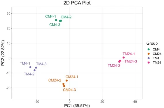
Batch effects are often first diagnosed using PCA, where samples may cluster by batch rather than by biological condition. Correction can be performed using methods such as ComBat, which applies empirical Bayes adjustment, or functions like removeBatchEffect in limma. Importantly, computational correction is most effective when combined with sound experimental design, especially ensuring that biological groups are evenly distributed across batches.

3.3 Missing Value Imputation

Missing values are a common feature of quantitative proteomics, particularly in DDA-LFQ where precursor sampling is stochastic and low-abundance peptides may fall below detection. Missingness can be categorized as MCAR, MAR, or MNAR; in proteomics, missing values often behave like MNAR, where absence correlates with low abundance.

A typical strategy starts with filtering, removing proteins with excessive missingness and retaining those supported by sufficient observations within at least one group. Remaining missing values can be imputed using methods aligned to the missingness mechanism. For MNAR-like patterns, a common approach is imputing from a low-intensity distribution, as implemented in Perseus through “Impute from normal distribution,” which shifts the mean downward and narrows the variance. For MAR/MCAR-like patterns, methods such as kNN, PCA-based imputation, or Bayesian PCA may be used. Tools including Perseus, MSstats, and R packages such as MSnbase offer flexible options for missing-value processing.

3.4 Statistical Significance Analysis

Once the data matrix has been normalized and refined, statistical testing identifies proteins with significant abundance differences between experimental conditions. Standard approaches include t-tests for two-group comparisons (often Welch’s t-test to relax equal-variance assumptions), ANOVA for multi-group settings, and linear-model frameworks.

A widely used option in omics is limma, which applies empirical Bayes moderation to stabilize variance estimates and increase power, particularly when sample size is limited. Because proteomics routinely tests thousands of proteins, multiple testing correction is essential. The Benjamini–Hochberg procedure is commonly used to control FDR, with typical significance criteria combining an adjusted q-value threshold (for example < 0.05 or 0.01) and a fold-change cutoff (for example 1.5× or 2×), depending on study goals.

Visualization helps communicate both statistical significance and biological effect size. Volcano plots summarize fold change against adjusted significance, while heatmaps reveal expression patterns across samples and highlight clustering behavior driven by differential proteins.

4. Functional Interpretation of Proteomics Results: Enrichment and Pathway Analysis

Differential protein lists become more interpretable when mapped to biological functions, pathways, and coordinated gene sets. Functional enrichment analysis is therefore a core step in turning proteomics outputs into mechanistic hypotheses.

4.1 GO enrichment analysis (Gene Ontology)

GO enrichment is a foundational approach that categorizes proteins across three ontologies: Biological Process (BP), Molecular Function (MF), and Cellular Component (CC). In practice, differential proteins are first mapped to GO terms using appropriate identifiers (often UniProt IDs), followed by statistical testing such as Fisher’s exact test or a hypergeometric test. Results are usually summarized by reporting the most significant terms (commonly top 10–20), providing a compact view of overrepresented functions and cellular localizations. (Learn more at: GO vs KEGG vs GSEA: How to Choose the Right Enrichment Analysis?)

4.2 KEGG pathway enrichment analysis

KEGG pathway analysis places differential proteins into curated biochemical and signaling pathways, supporting interpretation at the network level rather than focusing on individual proteins. Core concepts include pathway membership and KEGG Orthology (KO) identifiers, which group functionally equivalent proteins across species. The typical workflow maps proteins to KEGG pathways, performs enrichment testing (often Fisher’s exact test), and reports the most significantly enriched pathways to highlight biological themes such as signaling cascades, metabolic shifts, or stress responses.

4.3 COG/KOG enrichment analysis

COG/KOG annotation is particularly common in microbial proteomics and comparative analyses, classifying proteins into evolutionarily conserved functional categories. In many workflows, sequences are aligned against COG/KOG databases to assign functional groups, and enrichment is summarized by comparing the distribution of differential proteins across categories such as metabolism, information processing, and cellular processes.

4.4 GSEA enrichment analysis

Gene Set Enrichment Analysis (GSEA) differs from traditional over-representation analysis by using ranked data rather than strict cutoffs. Instead of selecting only “significant” proteins, GSEA evaluates whether members of a predefined gene set cluster toward the top or bottom of a ranked list (often ranked by log2 fold change). This threshold-free design is especially useful when the number of differential proteins is small or individual changes are modest, yet coordinated shifts occur at the pathway level. Enrichment Score (ES) curves provide intuitive directionality, indicating whether a process is globally upregulated or downregulated.

4.5 Recommended data sources and tools

Reliable enrichment depends on high-quality annotations and well-maintained databases. Commonly used sources include UniProt for sequences and functional notes, KEGG for pathway definitions and KO mapping, NCBI COG for homologous groups, and the GO Consortium for ontology terms.

For implementation, the R package clusterProfiler is widely used for GO/KEGG enrichment and GSEA, while visualization-oriented tools include enrichShiny. Online platforms such as enrichR, g:Profiler, and Metascape provide convenient interfaces and multi-database support when rapid exploration is needed.

4.6 Visualization and interpretation

Visualization is often the bridge between enrichment statistics and biological storytelling. Bar plots summarize top enriched terms, while bubble plots simultaneously encode enrichment significance and the number of mapped proteins. Heatmaps connect functional results back to quantitative patterns across samples, and GSEA plots provide a clear view of enrichment direction and where gene-set members sit within the ranked list.

Reference

1. Chambers, M. C., Maclean, B., Burke, R., Amodei, D., Ruderman, D. L., Neumann, S., Gatto, L., Fischer, B., Pratt, B., Egertson, J., Hoff, K., Kessner, D., Tasman, N., Shulman, N., Frewen, B., Baker, T. A., Brusniak, M. Y., Paulse, C., Creasy, D., Flashner, L., … Mallick, P. (2012). A cross-platform toolkit for mass spectrometry and proteomics. Nature biotechnology, 30(10), 918–920. https://doi.org/10.1038/nbt.2377

2. Gao, Y., Gao, L., Kang, Y., Yang, G., Zhao, Z., Zhao, Y., & Li, S. (2024). Non-Targeted Metabolomics Analysis Reveals Metabolite Profiles Change During Whey Fermentation with Kluyveromyces marxianus. Metabolites, 14(12), 694. https://doi.org/10.3390/metabo14120694

3. Demichev, V., Messner, C. B., Vernardis, S. I., Lilley, K. S., & Ralser, M. (2020). DIA-NN: neural networks and interference correction enable deep proteome coverage in high throughput. Nature methods, 17(1), 41–44. https://doi.org/10.1038/s41592-019-0638-x

4. Ting, L., Cowley, M. J., Hoon, S. L., Guilhaus, M., Raftery, M. J., & Cavicchioli, R. (2009). Normalization and statistical analysis of quantitative proteomics data generated by metabolic labeling. Molecular & cellular proteomics: MCP, 8(10), 2227–2242. https://doi.org/10.1074/mcp.M800462-MCP200

5. O'Connell, J. D., Paulo, J. A., O'Brien, J. J., & Gygi, S. P. (2018). Proteome-Wide Evaluation of Two Common Protein Quantification Methods. Journal of proteome research, 17(5), 1934–1942. https://doi.org/10.1021/acs.jproteome.8b00016

6. Kim, J., Yoon, S., & Nam, D. (2020). netGO: R-Shiny package for network-integrated pathway enrichment analysis. Bioinformatics (Oxford, England), 36(10), 3283–3285. https://doi.org/10.1093/bioinformatics/btaa077