Candidate metabolites, proteins, lipids, and prediction models usually produce continuous measurements or probabilities rather than direct case-control decisions. ROC curve analysis shows how sensitivity and false-positive rate change across classification thresholds. A high area under the curve (AUC), however, does not by itself establish biomarker reliability or practical utility. Interpretation also depends on the outcome definition, score direction, cutoff objective, calibration, and validation design. This guide covers ROC fundamentals, AUC interpretation, cutoff selection, leakage-safe validation, R and Python implementation, and applications in metabolomics and multi-omics research.
1. ROC Curve Fundamentals: Scores, Outcomes, Sensitivity, and Specificity
ROC analysis requires a binary reference outcome and a continuous biomarker or model score. Examples include disease versus control paired with a metabolite concentration, biomarker ratio, predicted probability, or machine-learning score.
1.1 Continuous Scores, Binary Outcomes, and Positive-Class Direction
ROC analysis links a binary reference outcome with a continuous biomarker or model score. The outcome may be disease versus control, responder versus non-responder, or another predefined phenotype, while the score may be a metabolite concentration, biomarker ratio, predicted probability, or machine-learning output. Before calculation, define which class is positive and whether higher or lower values indicate that class. An incorrect direction can invert the curve and produce an AUC below 0.5, although a genuine inverse biological association can produce the same pattern and should be interpreted rather than automatically reversed. For a multivariable panel, the included variables must be combined by a defined model that generates one score per sample; separate univariate ROC curves cannot simply be averaged or merged.
1.2 Sensitivity, specificity, and the confusion matrix.
At any selected threshold, the continuous score is converted into a positive or negative classification, producing true positives (TP), false positives (FP), true negatives (TN), and false negatives (FN). Sensitivity, or the true-positive rate (TPR), is TP/(TP + FN) and describes the proportion of positive samples detected. Specificity is TN/(TN + FP) and describes the proportion of negative samples correctly rejected. The false-positive rate (FPR), which forms the ROC x-axis, is 1 - specificity. Changing the threshold changes all four confusion-matrix counts, which is why sensitivity and specificity should always be interpreted at a stated cutoff rather than as fixed properties of a biomarker.
2. How to Read a ROC Curve and Interpret AUC Correctly
A ROC curve summarizes the trade-off between detecting positive samples and incorrectly classifying negative samples.
Axes, reference line, and operating points. The horizontal axis shows the false-positive rate and the vertical axis shows the true-positive rate. The diagonal from (0, 0) to (1, 1) represents no useful ranking ability, while a curve that rises toward the upper-left region generally indicates stronger discrimination. Every point on the curve corresponds to a threshold, not to an individual sample. Lowering the threshold usually identifies more positive samples but also increases false positives; raising it typically improves specificity at the cost of additional false negatives. The position chosen for practical use is therefore an operating point that reflects a particular balance between the two types of error.
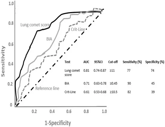
Figure 1. Example ROC curves showing the no-skill reference, AUC with 95% confidence intervals, and cutoff-specific sensitivity and specificity. Reproduced from Roumeliotis et al. (2022) under CC BY 4.0.
What AUC measures. AUC summarizes the ability of a score to rank positive samples above negative samples across all possible thresholds. With the direction defined correctly, it can be interpreted as the probability that a randomly selected positive sample receives a higher score than a randomly selected negative sample, with ties receiving half credit. An AUC of 0.5 indicates no ranking advantage over chance, whereas 1.0 indicates perfect separation (Hassanzad & Hajian-Tilaki, 2024). AUC is a population-level discrimination measure rather than the probability that any individual prediction is correct. Fixed labels such as “acceptable” or “excellent” should therefore not replace scientific context: case mix, disease spectrum, analytical conditions, and population differences can all change the observed value even when prevalence itself does not directly determine AUC.
Confidence intervals and model comparison. AUC should be reported with a 95% confidence interval because a point estimate alone does not show uncertainty. Wide intervals may reflect a small sample size, limited numbers in one outcome class, or heterogeneous data. DeLong's method and bootstrap resampling are commonly used to estimate uncertainty. When two models are evaluated on the same samples, their ROC curves are correlated and should be compared with a paired method such as the DeLong test (DeLong et al., 1988). Even a statistically significant increase in AUC may be too small to justify greater model complexity or laboratory burden, so comparison should also consider calibration, analytical reliability, reproducibility, and independent validation.
What AUC does not show. AUC does not assess probability calibration, identify a deployment cutoff, quantify positive or negative predictive value, account for unequal consequences of false-positive and false-negative decisions, or establish clinical utility. A model can rank samples correctly while systematically overestimating or underestimating absolute risk (Van Calster et al., 2019). For that reason, AUC should be interpreted together with confidence intervals, cutoff-specific metrics, calibration when probabilities are reported, and decision-oriented evidence when the model is intended to guide action.
Complementary metrics for imbalanced outcomes and probability prediction. ROC/AUC measures discrimination but does not describe every aspect of prediction performance. When positive outcomes are rare and the reliability of positive predictions is central, a precision-recall curve can complement ROC analysis by emphasizing precision and recall, although its interpretation depends on prevalence (Saito & Rehmsmeier, 2015). When model outputs are intended as probabilities, calibration should also be assessed to determine whether predicted risks agree with observed outcomes. The Brier score can provide a complementary measure of overall probabilistic error, but it should not be interpreted as a pure calibration metric (Van Calster et al., 2019).
Extensions beyond ordinary binary ROC analysis. The standard ROC framework assumes a binary outcome without censoring. Multiclass problems may require one-versus-rest class-specific curves together with clearly reported macro- or micro-averaged AUCs. For prognosis or other time-to-event outcomes, ordinary binary ROC analysis can ignore follow-up time and censoring; time-dependent ROC methods are more appropriate for evaluating discrimination at clinically relevant time points (Heagerty et al., 2000).
3. Step-by-Step ROC Curve Analysis Workflow for Omics Studies
Reliable ROC analysis is part of a complete prediction workflow in which data preparation, score generation, threshold selection, and validation are planned together.
3.1 Define the Outcome, Positive Class, Score Direction, and Intended Use
Define the binary endpoint, reference standard, positive class, score direction, and intended use, such as screening, diagnosis, prognosis, treatment-response prediction, or phenotype classification.
The intended use determines which errors matter most: screening may prioritize sensitivity, whereas confirmatory testing may prioritize specificity. Specify eligibility criteria and check whether batch, center, storage time, or sample source is confounded with the outcome.
3.2 Prepare the Data and Separate Development from Validation
Development data are used to fit preprocessing, select features, tune the model, and choose a candidate cutoff. Held-out and external-validation data must not influence these decisions.
Missing-value imputation, normalization, scaling, feature filtering, and feature selection should be performed within each training fold; applying them to the full dataset before cross-validation introduces information leakage. Nested cross-validation is useful when feature selection and tuning are performed together. Batch-correction methods also require care if they jointly use training and validation distributions. External validation provides the clearest assessment of transportability, and all development and validation steps should be reported transparently (Lewis et al., 2023; Bernett et al., 2024; Collins et al., 2024).
3.3 Build Prediction Scores and Construct the ROC Curve
For a single biomarker, the measured concentration or ratio may serve directly as the prediction score. A multivariable panel instead requires a defined algorithm, such as logistic regression, penalized regression, or random forest, that combines the selected variables and generates one score for each sample. The entire pipeline - including preprocessing, feature selection, and model fitting - should be treated as part of the model rather than as a collection of separate analyses.
The resulting model-derived score, rather than the individual ROC curves of its component biomarkers, is used for evaluation. Performance should be estimated from out-of-fold, held-out, or independent predictions rather than fitted training values, which usually describe optimistic apparent performance.
The ROC curve is then constructed by comparing each score with a sequence of candidate thresholds. Every threshold creates a new confusion matrix and therefore a new pair of TPR and FPR values. Plotting these pairs produces the operating points that make up the curve.
When larger scores indicate positivity, a very high threshold classifies almost every sample as negative, so both TPR and FPR approach zero. As the threshold decreases, sensitivity increases because more positive samples are detected, but false positives may also increase. At a very low threshold, nearly all samples are classified as positive and both rates approach one. This movement explains why no single point on the curve can be interpreted without its threshold and intended use.
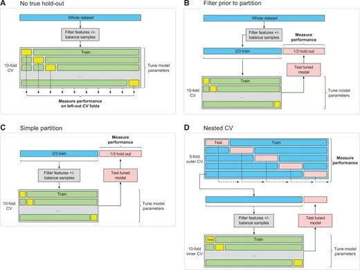
Figure 2. Classification thresholds generate different ROC operating points; the selected cutoff determines the corresponding sensitivity and specificity. Reproduced from Roumeliotis et al. (2022) under CC BY 4.0.
3.4 Select and Validate a Meaningful ROC Cutoff
The ROC curve contains many possible cutoffs. A common exploratory criterion is the Youden index:
J = sensitivity + specificity - 1
Maximizing J balances sensitivity and specificity but does not account for prevalence or unequal error costs, so it is not universally optimal (Youden, 1950; Hassanzad & Hajian-Tilaki, 2024).
Table 1. ROC Cutoff Selection Strategies: Objectives, Use Cases, and Limitations
| Strategy | Main objective | Suitable context | Main limitation |
|---|---|---|---|
| Youden index | Balance sensitivity and specificity | Exploratory biomarker evaluation | Ignores prevalence and unequal error costs |
| Sensitivity target | Reduce false negatives | Screening or rule-out use | May increase false positives |
| Specificity target | Reduce false positives | Confirmatory or rule-in use | May increase false negatives |
| Cost- or utility-based cutoff | Minimize expected consequences | Decision-oriented applications | Requires credible cost or utility assumptions |
Because prevalence affects PPV and NPV, these metrics should be interpreted for the intended population. Select the candidate cutoff in development data, lock it, and evaluate it unchanged in held-out or external data.
3.5 Lock the Model and Validate Performance in Held-Out or External Data
After development, refit the prespecified pipeline on the complete development cohort if appropriate, then lock preprocessing, feature strategy, model parameters, score direction, and cutoff. Apply the locked pipeline to held-out or external data without tuning, feature reselection, or cutoff adjustment.
Report AUC with its 95% confidence interval and performance at the fixed cutoff, including sensitivity and specificity and, where meaningful, PPV and NPV for the intended population. Calibration should be reported when model outputs are intended as probabilities, while precision-recall metrics may complement ROC analysis when positive outcomes are rare. The minimum information required for transparent reporting is summarized in Table 2 (Collins et al., 2024).
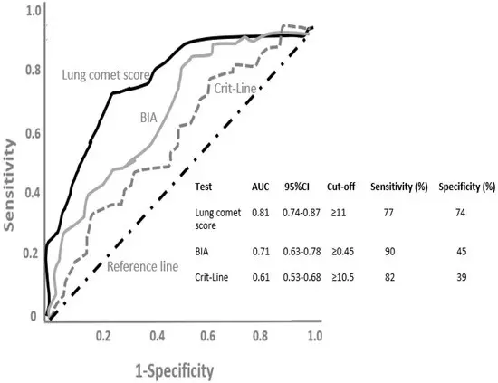
Figure 3. Biased and leakage-safe validation schemes for high-dimensional omics models. Reproduced from Lewis et al. (2023) under CC BY 4.0.
4. How to Perform ROC Curve Analysis in R and Python
R and Python should produce the same or nearly identical AUC when outcome coding, positive class, score direction, and tie handling are aligned. Threshold tables may differ slightly across packages. The examples assume outcome 1 is positive and larger scores indicate a higher likelihood of the positive class.
4.1 Input Data, Outcome Coding, and Positive-Class Definition
The example below contains ten simulated samples. Outcome 0 denotes the negative class and outcome 1 denotes the positive class, while higher biomarker scores are assumed to indicate a greater likelihood of the positive class. The two score distributions overlap - for example, the negative sample S05 has a higher score than the positive sample S06 - so the example demonstrates useful but imperfect discrimination rather than an unrealistic AUC of 1.0.
| Sample | Outcome | Biomarker score |
|---|---|---|
| S01 | 0 | 0.20 |
| S02 | 0 | 0.35 |
| S03 | 0 | 0.45 |
| S04 | 0 | 0.55 |
| S05 | 0 | 0.70 |
| S06 | 1 | 0.40 |
| S07 | 1 | 0.60 |
| S08 | 1 | 0.65 |
| S09 | 1 | 0.75 |
| S10 | 1 | 0.85 |
These simulated values are used only to demonstrate the calculations and should not be interpreted as diagnostic evidence. Formal evaluation should rely on predictions from samples that were not used to fit the corresponding model, such as out-of-fold, held-out, or external predictions.
4.2 ROC Curve Analysis in R with pROC
The pROC package supports ROC construction, AUC, confidence intervals, cutoff extraction, and curve comparison (Robin et al., 2011).
library(pROC)

df <- data.frame(
  outcome = c(0, 0, 0, 0, 0, 1, 1, 1, 1, 1),
  score = c(0.20, 0.35, 0.45, 0.55, 0.70, 0.40, 0.60, 0.65, 0.75, 0.85)
)

roc_obj <- roc(
  response = df$outcome,
  predictor = df$score,
  levels = c(0, 1),
  direction = "<",
  quiet = TRUE
)

auc_value <- auc(roc_obj)
auc_ci <- ci.auc(roc_obj, method = "delong")

best_cutoff <- coords(
  roc_obj,
  x = "best",
  best.method = "youden",
  ret = c("threshold", "sensitivity", "specificity")
)

plot(roc_obj, legacy.axes = TRUE)
print(auc_value)
print(auc_ci)
print(best_cutoff)
Confirm the score direction before analysis and validate the selected cutoff in independent data.
4.3 ROC Curve Analysis in Python with scikit-learn
Scikit-learn provides roc_curve() and roc_auc_score() for binary ROC analysis (Pedregosa et al., 2011).
import numpy as np
import matplotlib.pyplot as plt
from sklearn.metrics import roc_curve, roc_auc_score, confusion_matrix

y_true = np.array([0, 0, 0, 0, 0, 1, 1, 1, 1, 1])
y_score = np.array([0.20, 0.35, 0.45, 0.55, 0.70, 0.40, 0.60, 0.65, 0.75, 0.85])

fpr, tpr, thresholds = roc_curve(
    y_true, y_score, pos_label=1, drop_intermediate=False
)
auc_value = roc_auc_score(y_true, y_score)

finite = np.isfinite(thresholds)
j = tpr[finite] - fpr[finite]
best_idx = np.argmax(j)
cutoff = thresholds[finite][best_idx]

pred = (y_score >= cutoff).astype(int)
tn, fp, fn, tp = confusion_matrix(y_true, pred, labels=[0, 1]).ravel()
sensitivity = tp / (tp + fn)
specificity = tn / (tn + fp)

plt.plot(fpr, tpr, label=f"ROC curve (AUC = {auc_value:.3f})")
plt.plot([0, 1], [0, 1], linestyle="--", label="No-skill reference")
plt.xlabel("False Positive Rate")
plt.ylabel("True Positive Rate")
plt.title("Receiver Operating Characteristic Curve")
plt.legend()
plt.show()

print(auc_value, cutoff, sensitivity, specificity)
Bootstrap confidence intervals should resample the correct experimental unit. The cutoff shown here is selected for demonstration and requires independent validation.
5. Applications of ROC Analysis in Metabolomics and Multi-Omics Research
In omics research, ROC analysis can evaluate individual molecular features and integrated prediction panels, but interpretation must remain tied to analytical quality, study design, and intended use.
From single metabolites to multi-omics biomarker panels. A single-metabolite ROC curve evaluates whether one measurement can rank predefined groups, which can be useful during candidate screening or analytical verification. A biomarker panel combines several molecular variables - and sometimes clinical covariates - into one model-derived score. Such panels should be developed and validated as complete pipelines, with fold-specific preprocessing and feature selection, and compared with relevant alternatives such as clinical-only, omics-only, and clinical-plus-omics models. An increase in AUC should be interpreted together with its confidence interval, calibration, model complexity, and reproducibility rather than treated as sufficient evidence that the added omics features improve practice. High discrimination also cannot compensate for unstable compound identification, inadequate quality control, batch effects, or confounding by medication, fasting status, center, or sample handling.
Treatment response, disease subtyping, and phenotype classification. ROC analysis can also evaluate responder versus non-responder classification, molecular or clinical disease subtypes, environmental exposure classes, and plant stress-sensitive versus stress-resistant phenotypes. In exploratory studies, these analyses can prioritize candidates and clarify which operating points might be relevant for follow-up experiments. Translational or operational claims require stronger evidence: the outcome must be defined prospectively, analytical performance must be verified, the threshold should be predefined, and the complete model should be tested in independent data. Even then, discrimination is only one part of evaluation; the practical value of a test depends on whether its use changes decisions, reduces error, or improves downstream outcomes.
6. Common ROC Analysis Pitfalls and Minimum Reporting Checklist
Several recurring errors can make an ROC curve look more convincing than the underlying evidence. The most important problems are listed below; Table 2 then summarizes the information needed for interpretation and reproducibility.
- Full-dataset preprocessing or feature selection. Using all samples to impute, normalize, filter, or select features before resampling allows information from evaluation samples to influence model development and can inflate performance.
- Training-set ROC. A curve calculated from fitted training values describes apparent performance, not independent predictive ability. Out-of-fold, held-out, or external predictions provide a more credible basis for evaluation.
- Cutoff reuse. Selecting a cutoff in a test set and then reporting sensitivity and specificity in the same data gives an optimistic threshold-specific estimate. The cutoff should be chosen during development and confirmed unchanged in validation data.
- Incomplete reporting. AUC without the positive class, score direction, confidence interval, sample size, class distribution, and validation design is difficult to interpret or reproduce.
- Overclaiming and selective reporting. A high AUC does not prove causality, clinical utility, or generalizability. Trying many models and presenting only the strongest result without transparent comparison further increases the risk of misleading conclusions.
Table 2. Minimum Reporting Checklist for ROC Curve Analysis
| Category | Minimum information |
|---|---|
| Outcome and data | Outcome definition, positive class, score direction, cohort source, sample size, and class distribution |
| Model development | Preprocessing, feature selection, algorithm, tuning strategy, and cutoff-selection method |
| Validation | Internal validation design; held-out or external validation; whether predictions are out-of-fold |
| Performance | AUC with 95% CI; fixed cutoff; sensitivity, specificity, PPV, NPV, confusion matrix, and calibration when applicable |
| Reproducibility | Software and package versions, random seed, code, and analysis parameters when available |
Transparent reporting helps distinguish reproducible evidence from an attractive but potentially biased curve (Collins et al., 2024).
7. ROC Curve Analysis FAQs
These FAQs address three recurring interpretation and validation questions.
Is an AUC of 0.8 always good?
Not necessarily. Its meaning depends on the outcome definition, case mix, measurement quality, intended use, comparator, and validation cohort. An AUC of 0.8 may be encouraging in exploratory screening but inadequate when false decisions have serious consequences. It should be interpreted with its 95% confidence interval, calibration, cutoff-specific sensitivity and specificity, and evidence from held-out or external validation rather than assigned a universal quality label.
Is the Youden index always the best cutoff?
No. It gives equal weight to sensitivity and specificity, which is convenient for exploratory analysis but may conflict with the actual purpose of the test. Screening often prioritizes sensitivity, confirmatory testing may prioritize specificity, and decision-oriented applications may require explicit error costs or utility assumptions. The selected criterion should therefore be justified before validation and the chosen cutoff should be applied unchanged to independent data.
Can one dataset support development and final evaluation?
A single dataset can support model development when resampling is correctly nested and every data-driven step remains inside the training folds. However, the same observations should not be used to make all preprocessing, feature-selection, tuning, and cutoff decisions and then be presented as final proof of performance. Out-of-fold estimates are useful for internal evaluation, but fixed-cutoff performance should ideally be confirmed in a locked held-out set or an independent external cohort.
8. Plan a Validation-Aware ROC Biomarker Study with MetwareBio
Reliable ROC analysis requires reproducible molecular measurements and validation-aware study design. MetwareBio supports LC-MS/MS metabolomics and lipidomics, analytical QC, biomarker screening, statistical modeling, multi-omics integration, and biological interpretation aligned with the study objective and validation plan.
Planning a biomarker study or revising a ROC workflow? Contact MetwareBio to discuss an appropriate strategy.
Contact UsRead More: Biomarker Validation and Omics Data Analysis
These articles cover the analytical workflow surrounding ROC analysis — from differential feature screening and dimensionality reduction to machine learning and biomarker research — providing the methodological context needed to design and evaluate omics biomarker studies.
A comprehensive overview of the biomarker research workflow in metabolomics, covering candidate discovery, validation strategies, and analytical quality control — the upstream context in which ROC curve analysis is applied.
Random forest models frequently generate the prediction scores evaluated by ROC curves. This guide covers ensemble learning principles, feature importance, and cross-validation strategies directly relevant to building robust biomarker panels.
A practical case study applying machine learning and ROC analysis to metabolomics biomarker discovery in chronic kidney disease, demonstrating how AUC, cutoff selection, and validation are used in a real disease context.
Before ROC analysis, researchers must identify candidate features through differential analysis. This guide explains how volcano plots combine fold change and statistical significance to screen biomarker candidates for downstream validation.
Principal component analysis is a foundational dimensionality reduction technique used before feature selection and model building. Understanding PCA helps ensure that the data entering ROC analysis is properly preprocessed and structured.
The choice between parametric and non-parametric methods for differential analysis — which feeds into ROC-based biomarker evaluation — depends on data distribution. This article covers the normality tests that guide method selection.
References
- Bernett, J., Blumenthal, D. B., Grimm, D. G., Haselbeck, F., Joeres, R., Kalinina, O. V., & List, M. (2024). Guiding questions to avoid data leakage in biological machine learning applications. Nature Methods, 21, 1444-1453. https://doi.org/10.1038/s41592-024-02362-y
- Collins, G. S., Moons, K. G. M., Dhiman, P., Riley, R. D., Beam, A. L., Van Calster, B., et al. (2024). TRIPOD+AI statement: Updated guidance for reporting clinical prediction models that use regression or machine learning methods. BMJ, 385, e078378. https://doi.org/10.1136/bmj-2023-078378
- DeLong, E. R., DeLong, D. M., & Clarke-Pearson, D. L. (1988). Comparing the areas under two or more correlated receiver operating characteristic curves: A nonparametric approach. Biometrics, 44(3), 837-845. https://doi.org/10.2307/2531595
- Hassanzad, M., & Hajian-Tilaki, K. (2024). Methods of determining optimal cut-point of diagnostic biomarkers with application of clinical data in ROC analysis: An update review. BMC Medical Research Methodology, 24(1), 84. https://doi.org/10.1186/s12874-024-02198-2
- Heagerty, P. J., Lumley, T., & Pepe, M. S. (2000). Time-dependent ROC curves for censored survival data and a diagnostic marker. Biometrics, 56(2), 337-344. https://doi.org/10.1111/j.0006-341X.2000.00337.x
- Lewis, M. J., Spiliopoulou, A., Goldmann, K., Pitzalis, C., McKeigue, P., & Barnes, M. R. (2023). nestedcv: An R package for fast implementation of nested cross-validation with embedded feature selection designed for transcriptomics and high-dimensional data. Bioinformatics Advances, 3(1), vbad048. https://doi.org/10.1093/bioadv/vbad048
- Pedregosa, F., Varoquaux, G., Gramfort, A., Michel, V., Thirion, B., Grisel, O., et al. (2011). Scikit-learn: Machine learning in Python. Journal of Machine Learning Research, 12, 2825-2830. https://jmlr.org/papers/v12/pedregosa11a.html
- Robin, X., Turck, N., Hainard, A., Tiberti, N., Lisacek, F., Sanchez, J.-C., & Müller, M. (2011). pROC: An open-source package for R and S+ to analyze and compare ROC curves. BMC Bioinformatics, 12, 77. https://doi.org/10.1186/1471-2105-12-77
- Roumeliotis, S., Abd ElHafeez, S., D’Arrigo, G., Fusaro, M., Leonardis, D., Mezzatesta, S., & Tripepi, G. (2022). Fundamentals and applications of the receiver operating characteristic curve analysis in the research of endothelial dysfunction in chronic kidney disease. Life, 12(9), 1402. https://doi.org/10.3390/life12091402
- Saito, T., & Rehmsmeier, M. (2015). The precision-recall plot is more informative than the ROC plot when evaluating binary classifiers on imbalanced datasets. PLOS ONE, 10(3), e0118432. https://doi.org/10.1371/journal.pone.0118432
- Van Calster, B., McLernon, D. J., van Smeden, M., Wynants, L., & Steyerberg, E. W. (2019). Calibration: The Achilles heel of predictive analytics. BMC Medicine, 17, 230. https://doi.org/10.1186/s12916-019-1466-7
- Youden, W. J. (1950). Index for rating diagnostic tests. Cancer, 3(1), 32-35. https://doi.org/10.1002/1097-0142(1950)3:1%3C32::AID-CNCR2820030106%3E3.0.CO;2-3